Construction 20.8.1. Let \(f\colon A\to B\) be a morphism of Waldhausen categories.
Recall that \(i_n\colon [n]\to [n+1]\) is the upper embedding defined through \(i\mapsto i+1\).
We form the pullback square below.
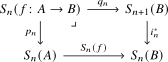 This construction clearly is functorial in \([n] : \Delta\catop\).
Proposition 20.8.2 (Waldhausen). Let \(C\) be an admissible class of Waldhausen
categories.
We consider a morphism \(f\colon A\to B\) in \(\WaldCat_C\).
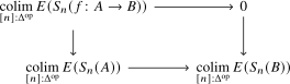
For any additive functor \(E\colon\WaldCat_C\to \An_{\bullet}\), there is a canonical
pullback square of the form below.
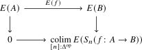
 In particular, there is a canonical fiber sequence of the form below.
Proof
The last assertion follows from the first by
Proposition 20.4.13. The proof of this proposition is in fact a variation on the proof
of the latter.
Since
\[
{\underset{[n] : \Delta\catop}{\colim}\, }E(\Scons_{n+1}(B))=0\, ,
\]
by Lemma 13.4.4, it suffices to prove that, for each \(n : \N\),
the induced commutative square
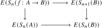 is a pullback square. Through the identifications \(\Scons_n(A)=A^{[n-1]}\) for \(n>0\),
one can identify \(\Scons_n(f\colon A\to B)\) as a category with terms the pairs \((x,y)\)
where \(x\) is a term in \(A^{[n-1]}\) and \(y\) a commutative diagram in \(B\) of the form
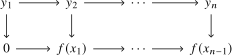 in which all squares are pushout squares.
Let \(v\colon \Scons_n(B)\hookrightarrow\Scons_{n+1}(B)\) be the full embedding
defined by sending a sequence
\[
x_1\to\cdots\to x_n
\]
to the sequence
\[
0\to x_1\to\cdots\to x_n\, .
\]
Since \(u\) is a section of \(i^*_n\), there is a canonical pullback square of the form below
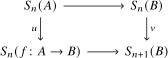 (in particular \(u\) is fully faithful and a section of \(p_n\)).
There is also a full embedding
\[
j\colon B\hookrightarrow\Scons_n(f\colon A\to B)
\]
defined by sending \(x\) to the pair consisting of the sequence of length \(n\)
\[
x\xrightarrow{\id_x}\cdots\xrightarrow{\id_x}x
\]
and of the commutative diagram
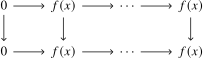 in which all the vertical maps are identities.
The functor \(j\) is a section of the functor \(\pi\) sending a pair \((x,y)\)
to the object \(y_1\). There is an obvious functorial exact sequence of the form
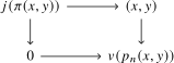 and therefore a direct application of Proposition 20.4.10
shows that the pair of functors
\[
(p_n,\pi)\colon\Scons_n(f\colon A\to B)\to \Scons_n(A)\times B
\]
induces an equivalence
\[
E(\Scons_n(f\colon A\to B))=
E(\Scons_n(A))\times E(B)\, .
\]
It follows that the squares
 are equivalent, hence are both cartesian, which achieves this proof.
Theorem 20.8.3 (Thomason-Trobaugh). Let \(B\) be a small stable category and \(A\) a thick subcategory of \(B\).
Then the pullback square
 induces a fiber sequence
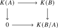 in \(\An_\bullet\).
Proof
We let \(C\) be the Waldhausen category defined by \(C=B\) as categories, with cofibrations being all maps but with weak equivalences being the maps whose cofiber lies in \(A\).
We observe then that the equivalence
\[
\Scons_{n+1}(B)=B^{[n]}
\]
induces an equivalence of the form
\[
\Scons_n(f\colon A\to B)=w_n(C)\, .
\]
Applying Proposition 20.8.2 to the admissible class of Waldhausen categories
given by small stable categories, with \(E=K\), and taking into account Remark 20.7.9,
we see that there is a canonical fiber sequence of the form
below.
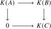 It suffices now to see that the morphism of Waldhausen categories
\(C\to B/A\) induced by the functor \(B\to B/A\) yields an equivalence of the form
\[
K(C)=K(B/A)\, .
\]
We want to understand the map
\[
{\underset{[m] : \Delta\catop}{\colim}\, } {\underset{[n] : \Delta\catop}{\colim}\, }
w_m(\Scons_{n}(C))^\simeq\to
{\underset{[m] : \Delta\catop}{\colim}\, } {\underset{[n] : \Delta\catop}{\colim}\, }
\Iso_m(\Scons_{n}(B/A))
\]
where \(\Iso_n=\Fun([n],(-)^\simeq)\).
The assignment
\[
[m]\mapsto w_m(\Scons_n(C))^\simeq
\]
is the nerve of the category of weak equivalences \(w(\Scons_n(C))\), whereas
\[
[m]\mapsto \Fun([m],\Scons_{n}(B/A)^\simeq)
\]
is the nerve of the anima \(\Scons_{n}(B/A)^\simeq\). Taking the colimit in the variable \([m]\)
amounts to consider the map
\[
\Pi_\infty(w(\Scons_n(C)))\to \Scons_{n}(B/A)^\simeq\, .
\]
It suffices to check that the latter is an equivalence for all \(n\).
The case \(n=0\) is obvious (we are comparing two terminal categories). For \(n>0\),
identifying \(\Scons_n\) with \((-)^{[n-1]}\), taking into account
Theorem 18.4.7
with \(P=[n-1]\), this is a particular case of Proposition 17.1.14.